

The end of running two databases. A step-by-step look at how we centralised all our monitoring in ClickHouse thanks to its new JSON type. Less infrastructure, queries up to 28x faster, and the lessons we learned in production.
Introduction and context
In one of our monitoring platforms, ClickHouse was already the primary data store for the metrics we collect at scale. However, our own telemetry (operating system statistics, Docker containers, database metrics, etc.) lived in a separate Telegraf + InfluxDB (1.8) stack. The reason was simple: Telegraf writes to InfluxDB using line protocol and everything is created automatically. A new host, a new container, a new field from a plugin? It simply appears. No schemas, no migrations, etc.
That convenience kept a second database alive for years. But two databases mean two systems to patch, monitor, back up and size, as well as two query languages in the same Grafana instance (where most of our dashboards and alerting rules live). All this while the platform’s primary data store — the one we already knew how to operate and scale — was sitting right next to it. We had wanted to consolidate everything into ClickHouse for a long time. What finally made it possible was ClickHouse’s native JSON data type (production-ready since version 25.3), which provides much of that schemaless development experience while retaining genuine columnar storage underneath.
In this article, we explain how we did it, the numbers we achieved, and what the JSON type costs at merge time — because nothing comes for free.
The JSON data type in ClickHouse
ClickHouse is a classic, strongly typed SQL database. Every column must be declared with an explicit type. Telegraf, on the other hand, emits dozens of measurements with hundreds of fields, and that set changes every time someone enables a plugin.
Before the native JSON type, mapping one world onto the other meant choosing between poor options.
You could mirror each Telegraf measurement in its own table, which meant writing and maintaining hundreds
of CREATE-TABLE statements and running ALTER-TABLE ADD COLUMN every time
a plugin added a field, leaving ingestion broken until someone did so. You could put everything into a
generic Map(String, Float64), which accepts anything but reads the entire map to access a
single key, giving up per-field compression and indexing. Or you could store the raw payload in aString column and parse it at query time, effectively throwing away the columnar engine
you came for.
The JSON type resolves that dilemma. The table declares a JSON column and needs nothing else; ClickHouse infers the fields from the data itself and stores them internally as real columns. You get InfluxDB’s “just send it” ergonomics on the write path and strict SQL performance on the read path.
The new solution
Telegraf continues to do the same job, but instead of writing to InfluxDB, it publishes JSON to Redpanda (essentially similar to Apache Kafka, for anyone unfamiliar with it). ClickHouse consumes it through a Kafka engine table and a couple of materialised views:
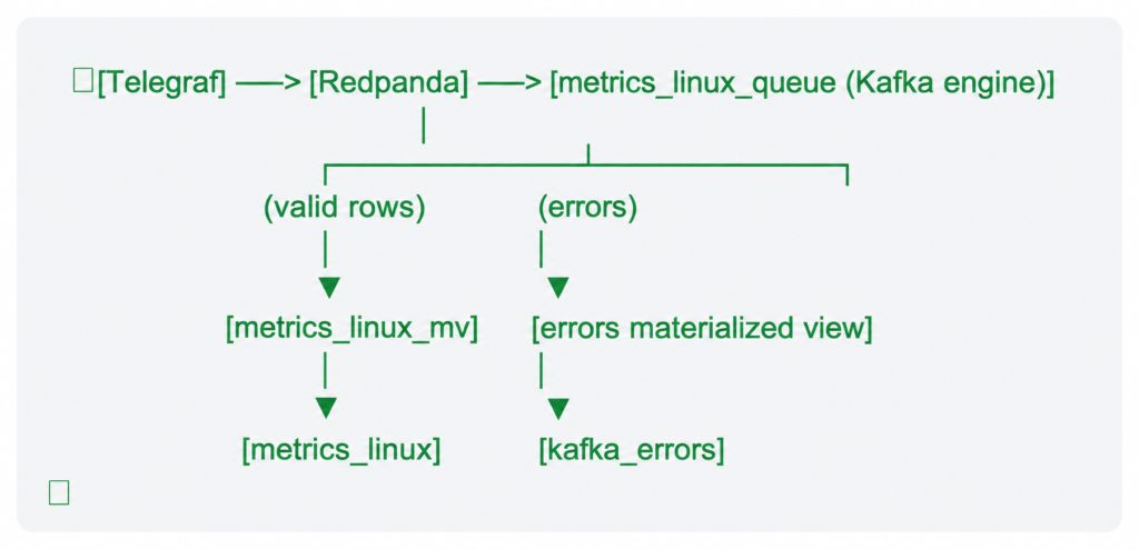
The Kafka engine table uses kafka_handle_error_mode = ‘stream’, so a malformed payload does not block the consumer: valid rows flow into the storage table, while invalid ones are sent to a dead-letter table together with the raw message and the associated parsing error. The consumer offset always moves forward.
The destination table is where things get interesting:
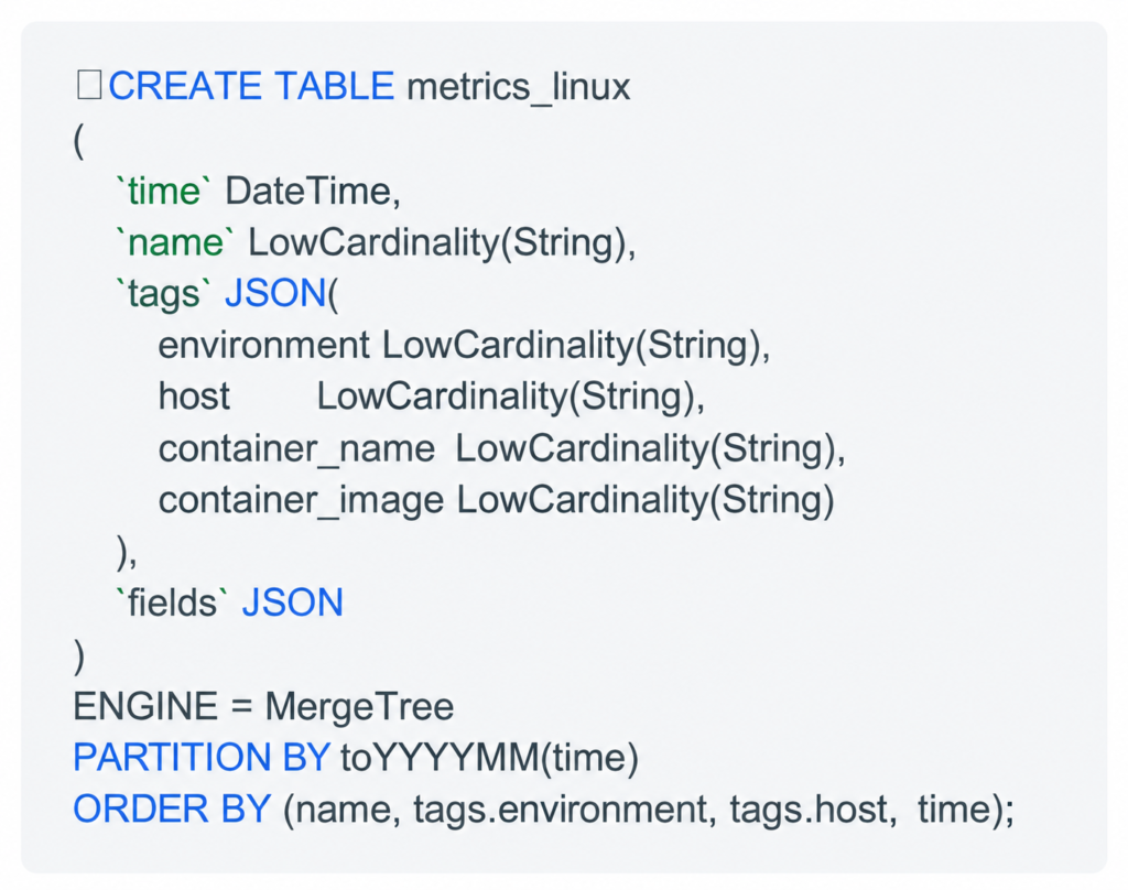
name contains what used to be the InfluxDB measurement (cpu, disk, docker_container_mem, …). Tags and fields are stored in two JSON columns. When a Telegraf plugin starts emitting a new field tomorrow, it will go straight into fields without anyone having to run an ALTER TABLE. That was precisely the point.
The JSON type
A JSON column in ClickHouse is not a string blob. On insert, ClickHouse parses each path (fields.usage_user, tags.host, …) and stores it as a real subcolumn, individually typed and compressed within the data part. Querying fields.usage_user reads only that subcolumn. It therefore has the same mechanics as a regular column and the same ability to be used in the primary key, as we do with tags.environment and tags.host in the ORDER BY.
There are three things worth knowing beyond the headline:
- Not everything has to be dynamic. You can provide type hints for paths you know will always be there, as we do with environment, host and the container tags. Hinted paths bypass type inference entirely and are stored using exactly that type. The documentation itself recommends providing hints for as many paths as possible; dynamic inference is the fallback for what cannot be predicted, not the default mode for everything. There are also SKIP and SKIP REGEXP clauses for discarding paths you will never query.
- There is a limit on dynamic paths, and the default is 1,024. Each JSON column stores at most max_dynamic_paths (1,024 by default) paths as real subcolumns per data part. Paths beyond that limit end up in a shared data structure (essentially a Map(String, String)) that remains queryable but is slower to read, because extracting a path may require scanning the map. During merges, if the combined parts exceed the limit, ClickHouse keeps the most frequently populated paths as subcolumns and moves the rarer ones into shared data. You can increase the setting, but the official recommendation is to proceed with caution: high values make storage and reads less efficient, with a suggested limit of around 10,000 for local disks and the default 1,024 for remote storage.
This limit shaped the design of our tables. Instead of one giant metrics table spanning every domain, we created one table per domain: metrics_linux, metrics_redpanda, metrics_postgres, metrics_grafana, etc. Our Redpanda brokers alone expose hundreds of different metric names; mixing fields from every domain into a single pair of JSON columns is the fastest way to exceed the path limit and have your most important metrics moved into shared data by the latest merge. Domain-specific tables keep each column’s path space small and predictable, and allow each table to have its own ORDER BY.
- Non-existent paths are read as NULL until you perform a cast. A dynamic subcolumn returns NULL for rows where the path is not present. But if you cast it to a plain Float64, those NULL values become 0.0, silently contaminating aggregations. Because Telegraf interleaves measurements in the same table, this becomes an immediate problem: avg(fields.load1::Float64) includes a zero in the average for every row containing fields from any other measurement. InfluxDB never exhibited this behaviour because it simply has no concept of that field existing at those points. The solution is to preserve NULL values as nullable when querying:
avg ignores NULL values, and the figures once again match InfluxDB. Filtering by name (and, where possible, by a field that always appears alongside the one you are aggregating) keeps these queries inexpensive.
The numbers
One clarification before we show the tables, because we prefer to err on the conservative side: our InfluxDB was an old 1.8 instance with years of accumulated data, running alongside other services; our ClickHouse is a recent version that also ingests much heavier, unrelated workloads. The time periods, hardware and workloads differ. None of this is a controlled benchmark. It is what we measured in our environment for Linux and Redpanda metrics, and the relative differences were large enough to absorb a generous margin of error.
Storage
Measured from system.parts (uncompressed bytes versus bytes on disk), on tables using the JSON type:
Telemetry domain | Compression ratio (raw → on disk) |
OS and Docker metrics | ~4.8× |
Redpanda broker metrics | ~58× |
Prometheus-style broker telemetry is brutally repetitive (the same sets of tags and very slowly changing counters, over and over again), and columnar storage combined with dictionary-encoded tag hints turns that redundancy into almost nothing. Comparing time windows of the same duration against what InfluxDB used for the equivalent database, we estimate roughly 3–4x less disk space for the Redpanda domain. InfluxDB’s TSM engine also compresses; it simply cannot exploit column-level locality in the same way a columnar engine can.
Queries
Two real Grafana panels over a 24-hour window, using semantically equivalent queries (InfluxQL’s non_negative_derivative function versus ClickHouse’s nonNegativeDerivative window function over JSON subcolumns):
Panel | InfluxDB 1.8 | ClickHouse 25.8 | Speed-up |
Rate (rate) of a gauge, 1-minute intervals, grouped by shard | ~200 ms | ~10 ms | ~20× |
Rate (rate) over a summed counter, 2-minute intervals, grouped by topic | ~3.4 s | ~0.12 s | ~28× |
The second panel is the interesting one: it performs aggregations across many series, which is precisely where InfluxDB 1.8’s per-series storage model becomes expensive, while a columnar scan with primary-key pruning (name, tags.environment, tags.host in the sorting key) barely notices.
The fine print: JSON merges devour RAM
ClickHouse writes inserts as immutable parts and continuously merges them in the background. For conventional fixed-schema tables, this is inexpensive. For JSON columns, it is not: a merge has to reconcile the dynamic subcolumn structure of every input part. It discovers the union of paths, rebuilds the columns for each path and the LowCardinality dictionaries, and decides what remains dynamic versus what is moved into shared data.
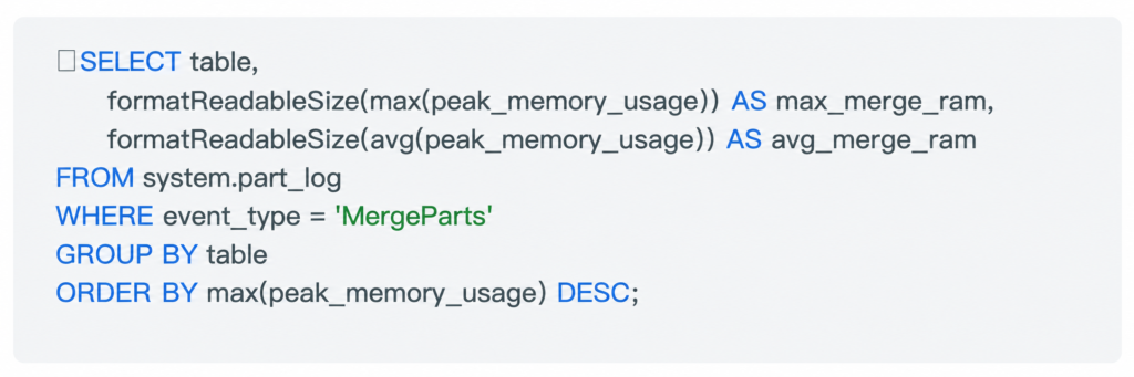
system.part_log records the peak memory usage of every historical merge, and the contrast in our cluster is stark:
Table | Schema | Peak RAM observed for a single merge |
Typical table containing other metric types in our monitoring platform | Simple typed columns | ~75 MiB (while merging ~5 GiB of raw data) |
metrics_linux | 2 JSON columns | ~2.8 GiB |
metrics_redpanda | 2 JSON columns | ~3.8 GiB |
The JSON tables therefore used far more memory to merge partitions. That is the price of schema flexibility, and it remains invisible until the day several of these merges run in parallel. For us, that day came when we started consuming from a Redpanda topic with a large accumulated backlog. Here is the chain of events, in case it saves you an afternoon:
- ClickHouse flushed thousands of tiny parts (a few hundred KiB each).
- The table triggered the TOO_MANY_PARTS circuit breaker (3,000 parts by default) and ingestion paused. So far, so good: that is backpressure doing its job, with the data waiting safely in Kafka.
- What did not go so well: the background pool (16 threads by default, overscheduled 2x by background_merges_mutations_concurrency_ratio) launched dozens of concurrent JSON merges, each requesting anything from hundreds of MiB to several GiB. In our setup (a development environment with less memory allocated), the merges piled up, hit the memory limit, were killed, rolled back and retried. An OOM loop that made no progress at all, while the memory manager’s OvercommitTracker killed innocent SELECT queries as collateral damage.
What actually fixed it:
- Limit merge concurrency: We sized background_pool_size according to the actual CPUs and set background_merges_mutations_concurrency_ratio = 1, so worst-case merge memory is simply the number of threads multiplied by peak RAM per merge — a figure you can budget for rather than discover the hard way. (If you reduce the pool, scale the MergeTree number_of_free_entries_in_pool_to_* settings proportionally, or the server will refuse to start).
- Real memory headroom: We sized the ClickHouse server resources based on the data measured in system.part_log. With JSON tables, we need to ensure there is enough memory not only when data arrives in a steady state, but also when there are large backlogs of data to process.
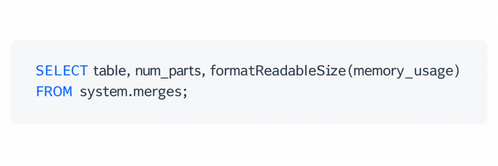
To help diagnose these issues, this query is useful for seeing exactly what is being merged right now:
Recent ClickHouse versions also include merge_max_dynamic_subcolumns_in_wide_part / merge_max_dynamic_subcolumns_in_compact_part to limit how many dynamic subcolumns are materialised by merges.
Conclusions
The JSON type delivers the InfluxDB/Telegraf experience on top of a columnar engine: new fields simply appear and can be queried at native-column speed. Compression on repetitive telemetry data ranges from very good to frankly absurd.
- Provide hints wherever you can. Type-hinted paths (especially LowCardinality tags used in the sorting key) are where most of the storage and query gains come from. If certain fields are always present, simply add the hint to the JSON type.
- Respect the budget of ~1,024 dynamic paths per JSON column. Scope tables by domain rather than increasing the limit; paths moved into shared data still work, but more slowly, and merges decide which ones get moved.
- Watch the semantics of casting NULL versus zero in sparse fields, or your averages will lie to you.
- Budget memory for merges, not just queries. A JSON-heavy table may need gigabytes for a single background merge that a fixed-schema table would handle with tens of megabytes. Measure it in system.part_log, limit concurrency and keep ingestion parts large.
One final note for transparency: we compared a current ClickHouse release with InfluxDB 1.8, which was several major versions behind. The difference would almost certainly be smaller against a modern InfluxDB. But this exercise was not only about performance. It was also about having one fewer database, a single query language for everything, and doing so without giving up schema flexibility.
Has this article made you rethink the efficiency of your own metrics architecture? We know every infrastructure is different and that the fine print matters. If you have any questions about what we have covered in this post, or if you need specialist advice on scaling, optimising or unifying your data platforms, feel free to contact us via LinkedIn or at https://datadope.io/contacto/

Óscar Erades de Quevedo.

